[5분 SOTA 논문 컨트리뷰션 리뷰 #7] CVPR 2015, Deep Residual Learning for Image Recognition

본 포스팅에서는 Deep Residual Learning for Image Recognition (CVPR 2015) 논문을 간단히 리뷰하였습니다.

 

모든 그림과 설명은 논문과 Stanford University CS231n Spring 2017 자료를 참고하였습니다.

 

원문 링크 : 

https://arxiv.org/abs/1512.03385

Deep Residual Learning for Image Recognition

---

1. Motivation

 

Stanford University CS231n Spring 2017 Lecture 9

 

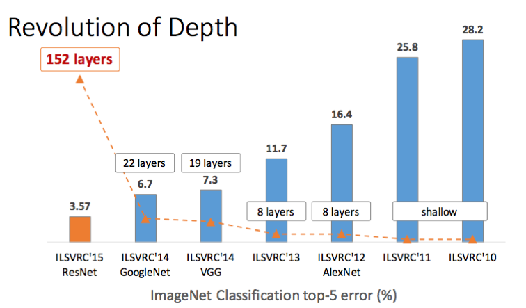
본 논문은 ImageNet Large Scale Visual Recognition Challenge에 우승한 model 연구를 바탕으로 layer의 depth를 깊게 한다면 성능이 향상될 것이라고 생각하며 연구를 시작하였습니다.

 

Figure 1. The deeper network has higher training error, and thus test error.

 

하지만 Model의 depth 가 깊어지면 깊어질수록 성능이 향상될 것이라 예상하였지만 반대로 성능이 떨어지는데 그 이유는 gradient vanishin/exploding 문제로 인하여 학습이 잘 이루어지지 않기 때문입니다.

 

본 논문에서는 이러한 문제를 해결하기 위하여 Shortcut connection을 이용한 residual learning을 통해 layer 가 깊어짐에 따른 gradient vanishing 문제를 해결하여 stat of the art 성능을 달성하였습니다.

 

2. Unique methodology 

 

1) Residual Learning

 

Figure 2. Residual learning: a building block.

 

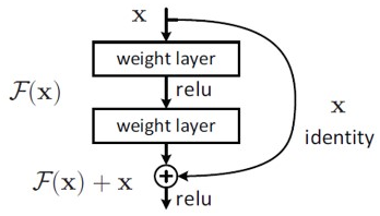
마지막에 이전 layer의 output인 x를 더하여 Network의 output은 0이 되도록 mapping 하여 최종 output이 x가 되도록 학습하면 layer가 증가하더라도 gradient로 1 이상의 값을 갖게 되어 gradient vanishing 문제를 해결하였습니다.

 

2) Network Architectures

 

Figure 3. Example network architectures for ImageNet. Left: the VGG-19 model [41] (19.6 billion FLOPs) as a reference. Middle: a plain network with 34 parameter layers (3.6 billion FLOPs). Right: a residual network with 34 parameter layers (3.6 billion FLOPs). The dotted shortcuts increase dimensions. Table 1 shows more details and other variants.

 

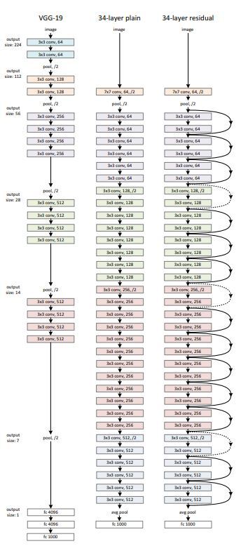
• ResNet은 VGG을 바탕으로 plain net을 만들었으며 동일한 feature map size를 갖게 하기 위해 layer에서 3*3 filter를 사용하였습니다. 또한 stride 2로 downsampling 할 때에는 channel 수를 두배로 늘려 time complexity를 유지하였습니다.
• 마지막 convolutional layer의 output은 global average pooling을 통해서 pooling을 하였습니다.
• 이러한 구조를 기반으로 하여 VGG보다 filter 개수를 낮추어 parmeter, complexity, 연산량을 낮추었습니다.

 

3. Results

 

Table 2. Top-1 error (%, 10-crop testing) on ImageNet validation. Here the ResNets have no extra parameter compared to their plain 

Figure 4. Training on ImageNet. Thin curves denote training error, and bold curves denote validation error of the center crops. Left: plain networks of 18 and 34 layers. Right: ResNets of 18 and 34 layers. In this plot, the residual networks have no extra parameter compared to their plain counterparts

Table 3. Error rates (%, 10-crop testing) on ImageNet validation. VGG-16 is based on our test. ResNet-50/101/152 are of option B that only uses projections for increasing dimensions.

Table 4. Error rates (%) of single-model results on the ImageNet validation set (except y reported on the test set).

Table 5. Error rates (%) of ensembles. The top-5 error is on the test set of ImageNet and reported by the test server.

Table 6. Classification error on the CIFAR-10 test set.

 

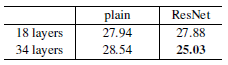
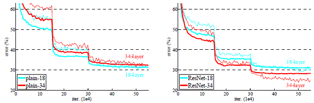
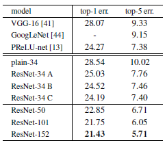
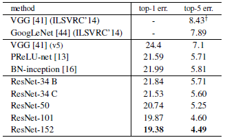
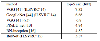
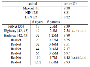
Table 2를 통해 알 수 있는 점은

• plain network의 경우 layer 가 깊은 model의 Top-1 error가 더 높은 반면 본 논문에서 제시한 model 인 ResNet 은 model의 깊이가 깊어질수록 Top-1 error 가 낮아지는 것을 확인할 수 있다.

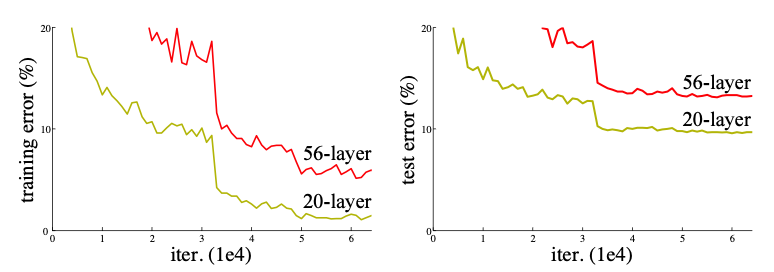
Figure 4를 통해 알 수 있는 점은

• 본 논문에서 제시한 model 인 ResNet 이  plain network 보다 수렴도 더 빨리 되며 ResNet model의 경우에는 model의 깊이가 깊어질수록 수렴하는 속도와 error 비율이 낮아진다.

Table 3, 4를 통해 알 수 있는 점은

• 기존의 다른 model 들과 비교하여 ResNet-152 가 Top-1, Top-5 error 면에서 가장 좋은 성능을 보여주고 있습니다.

Table 5를 통해 알 수 있는 점은

• ensembles을 사용한 ResNet 이 기존 state of the art model 보다 더 좋은 성능을 보여주고 있습니다.

Table 6를 통해 알 수 있는 점은

• 1202-layer network는 110-layer network와 비슷한 training error 보여주고 있지만, 실제 성능은 더 좋지 못합니다. 왜냐하면 Dataset의 크기에 비해 layer가 과도하게 많아서입니다.

 

FLOPS(FLoating point Operations Per Second)

: 컴퓨터가 1초 동안 수행할 수 있는 부동소수점 연산의 횟수를 기준으로 삼는다.